How to Reverse Case of Text in Excel

When importing data from another source, often times the data is displayed in all uppercase or all lowercase text. If you want to change the case, follow these instructions for Excel 2016 and 2013. (Terms may vary between versions, but the steps should remain the same.)

1. Next to the column or row that contains the text you would like to change, insert another column or row > Select the first cell in that column or row.
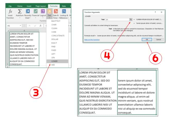
2. Select the "Formulas" tab > Select the "Text" drop-down list in the "Function Library" group.
3. Select "LOWER" for lowercase and "UPPER" for uppercase.
4. Next to the "Text" field, click the spreadsheet icon.
5. Click the first cell in the row or column that you would like to change the text case.
6. Click on the spreadsheet icon again in the "Function Arguments" pop-up > Click [OK].
7. In the cell where the text converted to the desired case, click the small square in the bottom right corner of the cell and drag down to convert the rest of the adjacent column or row's text.
8. When you have an entire column or row with the desired text, copy and past the text into the original column or row > Delete the duplicate column or row that you created in step 1.

Keywords: lower case, change words, no caps, all caps, office 2010